Types of Sensitivity Analysis
Categories of Sensitivity Analysis
- One-at-a-Time vs. All-At-A-Time Sampling
- Local vs. Global
One-At-A-Time SA
Assumption: Factors are linearly independent (no interactions).
Benefits: Easy to implement and interpret.
Limits: Ignores potential interactions.
All-At-A-Time SA
Number of different sampling strategies: full factorial, Latin hypercubes, more.
Benefits: Can capture interactions between factors.
Challenges: Can be computationally expensive, does not reveal where key sensitivities occur.
Local SA
Local sensitivities: Pointwise perturbations from some baseline point.
Challenge: Which point to use?
Global SA
Global sensitivities: Sample throughout the space.
Challenge: How to measure global sensitivity to a particular output?
Advantage: Can estimate interactions between parameters
How To Calculate Sensitivities?
Number of approaches. Some examples:
- Derivative-based or Elementary Effect (Method of Morris)
- Regression
- Variance Decomposition or ANOVA (Sobol Method)
- Density-based (\(\delta\) Moment-Independent Method)
Parameter Ranges
For a fixed release strategy, look at how different parameters influence reliability.
Take \(a_t=0.03\), and look at the following parameters within ranges:
| \(q\) |
\((2, 3)\) |
| \(b\) |
\((0.3, 0.5)\) |
| \(ymean\) |
\((\log(0.01), \log(0.07))\) |
| \(ystd\) |
\((0.01, 0.25)\) |
Method of Morris
The Method of Morris is an elementary effects method.
This is a global, one-at-a-time method which averages effects of perturbations at different values \(\bar{x}_i\):
\[S_i = \frac{1}{r} \sum_{j=1}^r \frac{f(\bar{x}^j_1, \ldots, \bar{x}^j_i + \Delta_i, \bar{x}^j_n) - f(\bar{x}^j_1, \ldots, \bar{x}^j_i, \ldots, \bar{x}^j_n)}{\Delta_i}\]
where \(\Delta_i\) is the step size.
Sobol’ Method
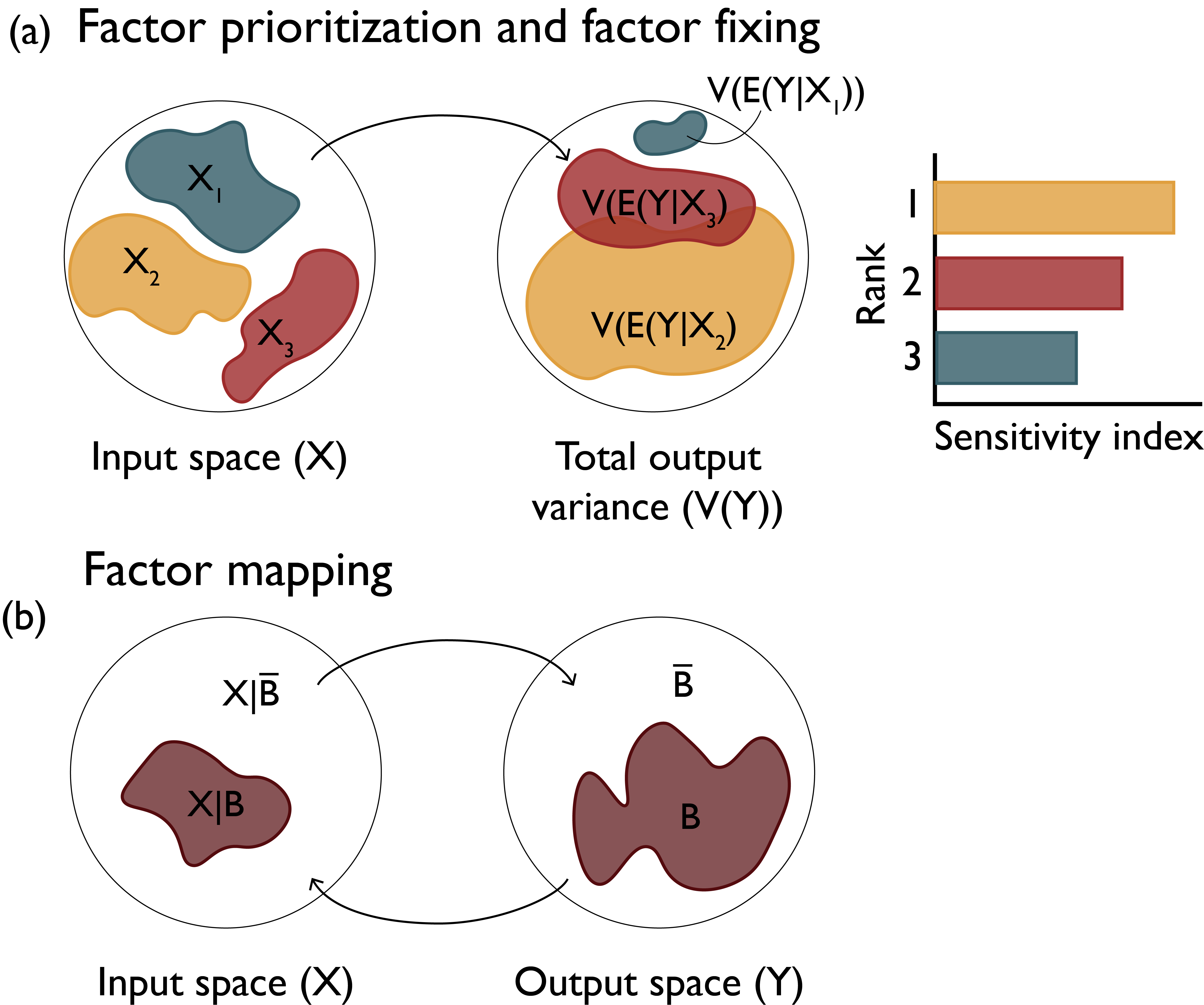
The Sobol method is a variance decomposition method, which attributes the variance of the output into contributions from individual parameters or interactions between parameters.
\[S_i^1 = \frac{Var_{x_i}\left[E_{x_{\sim i}}(x_i)\right]}{Var(y)}\]
\[S_{i,j}^2 = \frac{Var_{x_{i,j}}\left[E_{x_{\sim i,j}}(x_i, x_j)\right]}{Var(y)}\]
Sobol’ Method: First and Total Order
┌ Warning: The `generate_design_matrices(n, d, sampler, R = NoRand(), num_mats)` method does not produces true and independent QMC matrices, see [this doc warning](https://docs.sciml.ai/QuasiMonteCarlo/stable/design_matrix/) for more context.
│     Prefer using randomization methods such as `R = Shift()`, `R = MatousekScrambling()`, etc., see [documentation](https://docs.sciml.ai/QuasiMonteCarlo/stable/randomization/)
└ @ QuasiMonteCarlo ~/.julia/packages/QuasiMonteCarlo/KvLfb/src/RandomizedQuasiMonteCarlo/iterators.jl:255
Sobol’ Method: Second Order
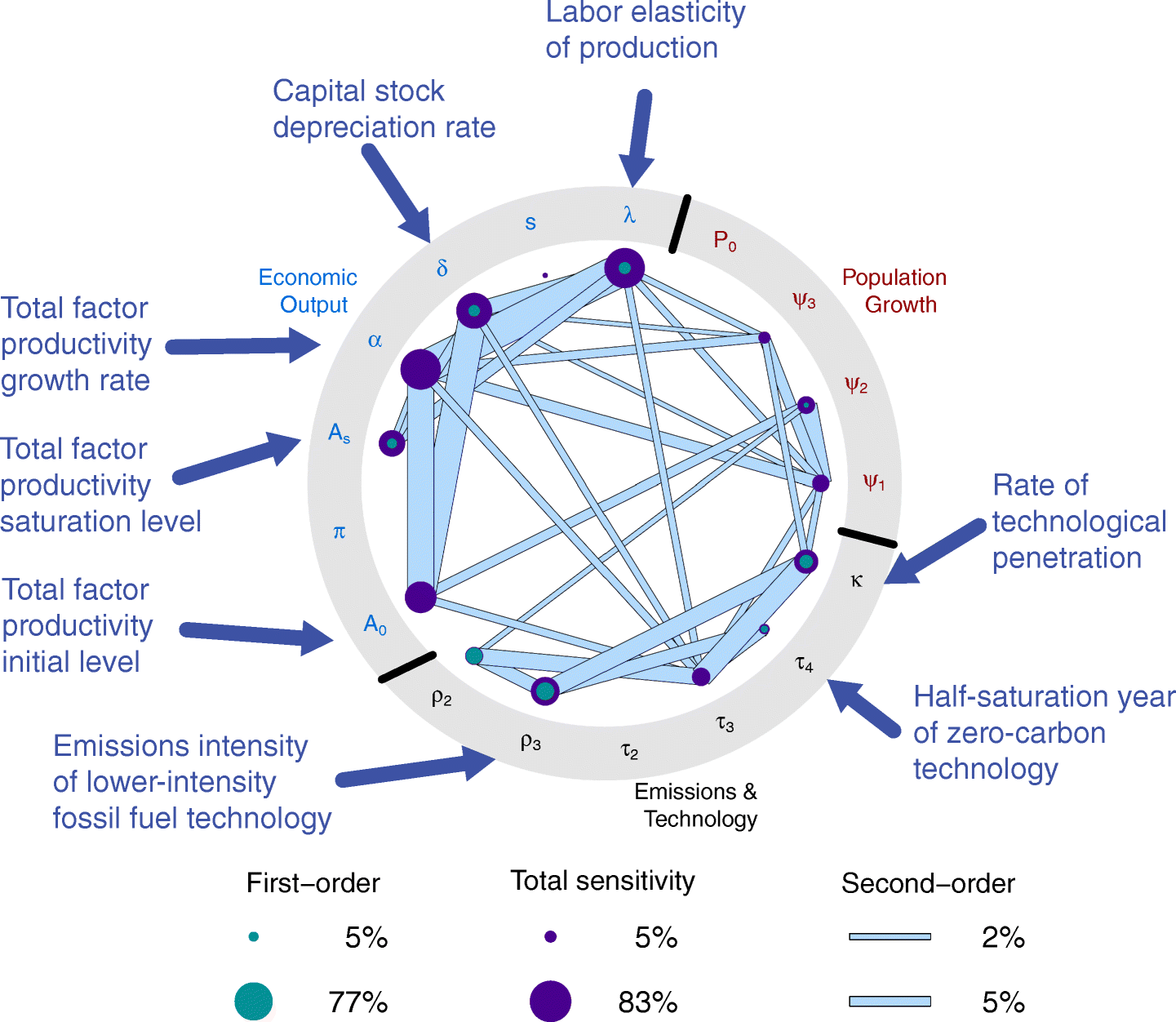
Example: Cumulative CO2 Emissions
![]()
Model for CO2 Emissions
Example: Cumulative CO2 Emissions
![]()
CO2 Emissions Sensitivities