| Generator | Fixed Cost ($) | Variable Cost ($/MW) |
|---|---|---|
| Geothermal | 450000 | 0 |
| Coal | 220000 | 21 |
| NG CCGT | 82000 | 25 |
| NG CT | 65000 | 35 |
Power Systems: Generating Capacity Expansion
Lecture 17
October 13, 2023
Review and Questions
Last Class
- Resource allocation problem as a linear program
- Worked land allocation example
Questions?

Text: VSRIKRISH to 22333
Electric Power System Decision Problems
Overview of Electric Power Systems

Power Systems Schematic
Source: Wikipedia
Decisions Problems for Power Systems

Decision Problems for Power Systems by Time Scale
Adapted from Perez-Arriaga, Ignacio J., Hugh Rudnick, and Michel Rivier (2009)
Electricity Generation by Source
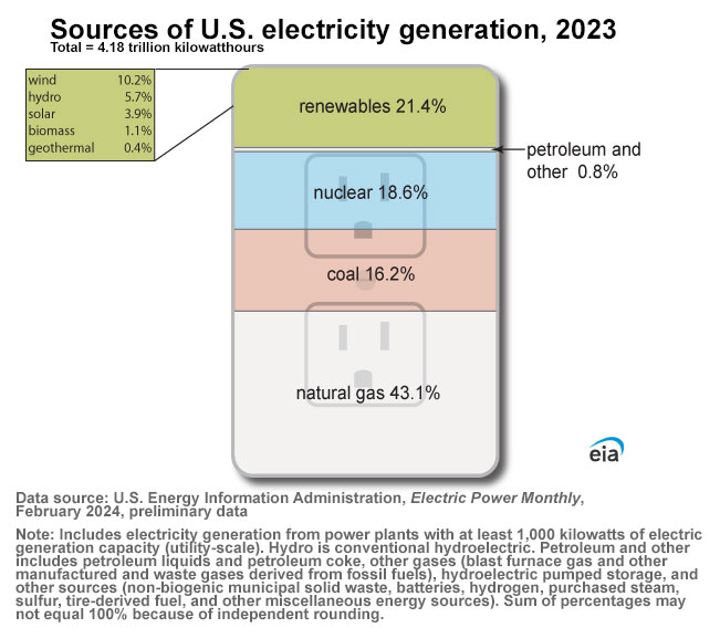
Electricity Generation in 2022 by Source
Source: U.S. Energy Information Administration
Generating Capacity Expansion
Capacity Expansion
Capacity expansion involves adding resources to generate or transmit electricity to meet anticipated demand (load) in the future.
Typical objective: Minimize cost
But other constraints may apply, e.g. reducing CO2 emissions or increasing fuel diversity.
Simple Capacity Expansion Example
Plant Types
In general, we have many fuel options:
- Gas (combined cycle or simple cycle);
- Coal;
- Nuclear;
- Renewables (wind, solar, hydro, geothermal)
Simplified Example: Generators
Simplified Example: Demand
Simplified Example: Load Duration Curve
Simplified Example: Load Duration Curve
Capacity Expansion: Goal
We want to find the installed capacity of each technology that meets demand at all hours at minimal total cost.
Although…
- For some hours with extreme load, is it necessarily worth it to build new generation to meet those peaks?
- Instead, assign a high cost \(NSECost\) to non-served energy (NSE). In this case, let’s set \(NSECost = \$9000\)/MWh
Decision Variables
What are our variables?
| Variable | Meaning |
|---|---|
| \(x_g\) | installed capacity (MW) from each generator type \(g \in \mathcal{G}\) |
| \(y_{g,t}\) | production (MW) from each generator type \(g\) in hour \(t \in \mathcal{T}\) |
| \(NSE_t\) | non-served energy (MWh) in hour \(t \in \mathcal{T}\) |
Capacity Expansion Objective
\[ \begin{align} \min_{x, y, NSE} Z &= {\color{red}\text{investment cost} } + {\color{blue}\text{operating cost} } \\ &= {\color{red} \sum_{g \in \mathcal{G}} \text{FixedCost}_g x_g} + {\color{blue} \sum_{t \in \mathcal{T}} \sum_{g \in \mathcal{G}} \text{VarCost}_g y_{g,t} + \sum_{t \in \mathcal{T}} \text{NSECost} NSE_t} \end{align} \]
What Are Our Constraints?
Text: VSRIKRISH to 22333
Capacity Expansion Constraints
- Demand: Sum of generated energy and non-served energy must equal demand \(d_t\).
- Capacity: Generator types cannot produce more electricity than their installed capacity.
- Non-negativity: All decision variables must be non-negative.
Problem Formulation
\[ \begin{align} \min_{x, y, NSE} \quad & \sum_{g \in \mathcal{G}} \text{FixedCost}_g x_g + \sum_{t \in \mathcal{T}} \sum_{g \in \mathcal{G}} \text{VarCost}_gy_{g,t} & \\ & \quad + \sum_{t \in \mathcal{T}} \text{NSECost} NSE_t & \\[0.5em] \text {subject to:} \quad & \sum_{g \in \mathcal{G}} y_{g,t} + NSE_t = d_t \qquad \qquad \forall t \in \mathcal{T} \\[0.5em] & y_{g,t} \leq x_g \qquad \qquad \forall g \in {G}, \forall t \in \mathcal{T} \\[0.5em] & x_g, y_{g,t}, NSE_t \geq 0 \qquad \qquad \forall g \in {G}, \forall t \in \mathcal{T} \end{align} \]
Capacity Expansion is an LP
- Linearity: costs assumed to scale linearly;
- Divisible: we model total installed capacity, not number of individual units
- Certainty: no uncertainty about renewables.
Real problems can get much more complex, particularly if we try to model making decisions under renewable or load uncertainty.
Capacity Expansion Example Solution
| Resource | Installed Capacity (MW) | Percent Installed (%) | Annual Generation (GWh) | Percent Generated (%) |
|---|---|---|---|---|
| Geothermal | 0.0 | 0.0 | -0.0 | -0.0 |
| Coal | 0.0 | 0.0 | -0.0 | -0.0 |
| NG CCGT | 2016.9 | 72.5 | 15157.7 | 98.1 |
| NG CT | 733.0 | 26.4 | 292.2 | 1.9 |
| NSE | 31.2 | 1.1 | 0.1 | 0.0 |
When Do Generators Operate?
What Does This Problem Formulation Neglect?
Text: VSRIKRISH to 22333
What Does This Problem Neglect?
- Discrete decisions: is a plant on or off (this is called unit commitment)?
- Intertemporal constraints: Power plants can’t just “ramp” from producing low levels of power to high levels of power; there are real engineering limits.
- Transmission: We can generate all the power we want, but what if we can’t get it to where the demand is
- Retirements: We might have existing generators that we want to retire (“brownfield” scenarios). ## What About Renewables?
Renewables make this problem more complicated because their capacity is variable:
- resource availability not constant across time;
- need to consider a capacity factor.
How would this change our existing capacity expansion formulation?
Renewable Variability Impact
This will change the capacity constraint from \[y_{g,t} \leq x_g \qquad \forall g \in {G}, \forall t \in \mathcal{T}\] to \[y_{g,t} \leq x_g \times c_{g,t} \qquad \forall g \in {G}, \forall t \in \mathcal{T}\] where \(c_{g,t}\) is the capacity factor in time period \(t\) for generator type \(g\).
Implementing Constraints in JuMP
I recommend using vector notation in JuMP to specify these constraints, e.g. for capacity:
# define sets
G = 1:num_gen # num_gen is the number of generators
T = 1:num_times # number of time periods

c = ... # G x T matrix of capacity factors
@variable(..., x[g in G] >= 0) # installed capacity
@variable(..., y[g in G, t in T] >= 0) # generated power
@constraint(..., capacity[g in G, t in T],
    y[g,t] <= x[g] * c[g,t]) # capacity constraint
Key Takeaways
Key Takeaways
- Capacity Expansion is a foundational power systems decision problem.
- Is an LP with some basic assumptions.
- We looked at a “greenfield” example: no existing plants.
- Decision problem becomes more complex with renewables (HW4) or “brownfield” (expanding existing fleet, possibly with retirements).
Upcoming Schedule
Next Classes
Monday: Economic Dispatch
Wednesday/Friday: Air Pollution
Assessments
- Lab 3 due tonight at 9pm.
- HW4 assigned Monday (likely over the weekend).