Uncertainty and Simple Climate Models
Lecture 12
September 22, 2023
Review and Questions
Monte Carlo
Monte Carlo is stochastic simulation.
Monte Carlo
Let \(Y=f(X)\), where \(X\) is a random variable. Let \(\mathbb{E}[Y] = \mu\).
If \(X_1, \ldots, X_n\) are independent samples, then the Monte Carlo estimate of \(\mu\) is \[\tilde{\mu}_n = \frac{1}{n} \sum_{i=1}^n f(X_i) = \frac{1}{n}\sum_{i=1}^n Y_i.\]
The key point: \(\tilde{\mu}_n \to \mu\) as \(n \to \infty\).
Monte Carlo Properties
Monte Carlo is an unbiased estimator: \[\mathbb{E}[\tilde{\mu}_n] = \mu.\]
Monte Carlo variance: \[\text{Var}[\tilde{\mu}_n] = \tilde{\sigma}_n^2 = \frac{\sigma_Y^2}{n}.\]
Monte Carlo Confidence Intervals
This means we can obtain \(\alpha\)-confidence intervals:
\[\tilde{\mu}_n \pm \Phi^{-1}\left(1 - \frac{\alpha}{2}\right) \frac{\sigma_Y}{\sqrt{n}}.\]
Questions?

Text: VSRIKRISH to 22333
Energy Balance and Climate Change
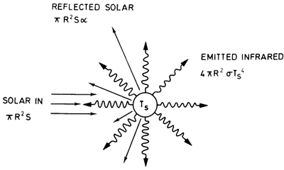
Planetary Energy Balance

Representation of Planetary Energy Balance
Source: Reprinted from A Climate Modeling Primer, A. Henderson-Sellers and K. McGuffie, Wiley, pg. 58, (1987) via https://www.e-education.psu.edu/meteo469/node/137.
Radiative Forcing
Climate changes result from changes to the energy balance of the planet (or radiative forcings), due to e.g.:
- greenhouse gas emissions (which trap radiation, warming the planet);
- aerosol emissions from air pollution or volcanic eruptions (which block incoming radiation, cooling the planet);
- changes to the solar cycle (which can increase or decrease the incoming solar radiation).
Historical and Projected Radiative Forcing
These projections are under RCP 8.5, which is the “worst-case” official future climate scenario.
Historical and Projected Radiative Forcing
These are RCP 2.6, one of the “better” scenarios (often a lower bound on future warming).
Global Mean Temperature
These radiative changes result in changes to global mean temperatures, which result in other impacts.
How can we model this relationship?
The Energy Balance Model (EBM)
Sketch of the EBM
- Simplest possible climate model.
- Treats the Earth as a 0-dimensional sphere covered with water.
- Earth warms due to imbalance in average (over surface area) heat flux.
EBM Equations
\[\begin{align*} \overbrace{\frac{dH}{dt}}^{\text{change in heat}} &= \overbrace{F}^{\text{RF}} - \overbrace{\lambda T}^{\substack{\text{change in} \\ \text{temperature}}} \\ \underbrace{C}_{\substack{\text{ocean heat} \\ \text{capacity}}} \frac{dT}{dt} &= F - \lambda T \\ c\underbrace{d}_{\substack{\text{ocean} \\ \text{mixing depth}}} \frac{dT}{dt} &= F - \lambda T, \end{align*}\]
EBM Equations
- \(c = 4.184\times 10^6 \\ \text{J/K/m}^2\) is the specific heat of water per area.
- Total RF: \[F = F_\text{non-aerosol} + \alpha F_\text{aerosol}.\]
- The proportionality coefficient \(\lambda\) is important: it is the climate feedback factor and controls how much the Earth warms in response to radiative forcing.
EBM Solution
We can solve the EBM using Euler timestepping:
\[\begin{gather*} C dT/dt = F - \lambda T \\\\ \Rightarrow C \frac{T_{i+1}-T_i}{\Delta t} = F_i - \lambda T_i \\\\ \Rightarrow T_{i+1} = T_i + \frac{F_i - \lambda T_i}{C} \Delta t \end{gather*}\]
What the EBM Neglects
The EBM is a one-box model of the Earth’s climate: models energy balance between incoming and outgoing heat. As such, it neglects:
- “Deep” ocean heat uptake and cycling.
- Multiple atmospheric layers.
- Spatial patterns of atmospheric and ocean circulation.
Equilibrium Climate Sensitivity (ECS)
Under steady-state conditions (constant \(F\) and \(dT/dt = 0\)), \[T = \frac{F}{\lambda}.\]
When we double atmospheric CO2, we refer to the equilibrium temperature \(S\) as the equilibrium climate sensitivity:
\[S = \underbrace{F_{2\times \text{CO}_2}}_{\approx 4 \text{W/m}^2}/\lambda\]
Equilibrium Climate Sensitivity Uncertainty
The ECS is very uncertain (though uncertainty has been reduced recently).
A reasonable distribution is \(S \sim \text{LogNormal}(\log(3.2), \log(2)/{3})\)
Best Fit EBM Simulation
Let’s run the EBM with typical values of \(S = 3.2^\circ\) C, \(d=100\)m, and \(\alpha = 1.3\).
Comparison to Temperature Data
How well does this do against the temperature data?
Monte Carlo Simulation and ECS Uncertainty
Uncertainty Propagation in the Climate System
How does uncertainty in the ECS propagate to uncertainty in temperatures in 2100?
Temperature Histograms
Uncertainty Propagation in the Climate System
Adding in temperature data…
Limits of the EBM Impact Parameterization
One of the problems is using parameter values/distributions which were chosen in a different context.
The EBM simplifies certain dynamics so much that these parameters, while they have physical interpretations, need different distributions or have different correlations.
Identifying these values for a particular model is called model calibration.
How Do We Make These Plots in Julia?
To compute quantiles and median, use
Distributions.quantile():Can broadcast quantile calculation over columns/rows of an array:
How Do We Make These Plots in Julia?
To plot intervals around a median (or other central value), use the
ribbon=keyword inplot()to pass an array of bounds. For example:
Key Points
Key Points
- Uncertainty propagation lets us quantify the impact of upstream uncertainties on system outputs
- Viewed the impact of climate sensitivity and radiative forcing uncertainty on temperature projections for a simple model.
- Distributions of uncertain inputs or parameters may not be directly usable in another model context due to model assumptions.
Upcoming Schedule
Next Classes
Next Week: Prescriptive Modeling and Optimization
Assessments
Today: Homework 2 and Lab 2 both due.
Monday: Homework 3 released (on uncertainty propagation from the EBM to sea-level rise and levee heights)
Next Friday: Project Proposal due