Why Monte Carlo Works
Lecture 11
September 20, 2023
Review and Questions
Monte Carlo Simulation
Monte Carlo is stochastic simulation.
Goals of Monte Carlo
Monte Carlo is a broad method, which can be used to:
- Obtain probability distributions of outputs (uncertainty propagation);
- Estimate deterministic quantities (Monte Carlo estimation).
Monte Carlo Estimation
Monte Carlo estimation involves framing the (deterministic) quantity of interest as a summary statistic of a random process.
Questions?

Text: VSRIKRISH to 22333
Monte Carlo: More Formally
Why Monte Carlo Works
We can formalize Monte Carlo estimation as the computation of the expected value of a random quantity \(Y\), \(\mu = \mathbb{E}[Y]\).
To do this, generate \(n\) independent and identically distributed values \(Y_1, \ldots, Y_n\). Then the sample estimate is
\[\tilde{\mu}_n = \frac{1}{n}\sum_{i=1}^n Y_i\]
Monte Carlo (Formally)
More generally, we want to compute some quantity \(Y=f(X)\), where \(X\) is distributed according to some probability distribution \(p(x)\) and \(f(x)\) is a real-valued function over a domain \(D\).
Then \[\mu = \mathbb{E}(Y) = \int_D f(x)p(x)dx.\]
The Law of Large Numbers
If
\(Y\) is a random variable and its expectation exists and
\(Y_1, \ldots, Y_n\) are independently and identically distributed
Then by the weak law of large numbers:
\[\lim_{n \to \infty} \mathbb{P}\left(\left|\tilde{\mu}_n - \mu\right| \leq \varepsilon \right) = 1\]
The Law of Large Numbers
In other words, eventually Monte Carlo estimates will get within an arbitrary error of the true expectation. But how large is large enough?
Note that the law of large numbers applies to vector-valued functions as well. The key is that \(f(x) = Y\) just needs to be sufficiently well-behaved.
Monte Carlo Sample Mean
The sample mean \(\tilde{\mu}_n = \frac{1}{n}\sum_{i=1}^n Y_i\) is itself a random variable.
With some assumptions (the mean of \(Y\) exists and \(Y\) has finite variance), the expected Monte Carlo sample mean \(\mathbb{E}[\tilde{\mu}_n]\) is
\[\frac{1}{n}\sum_{i=1}^n \mathbb{E}[Y_i] = \frac{1}{n} n \mu = \mu\]
So the Monte Carlo estimate is an unbiased estimate of the mean.
Monte Carlo Error
We’d like to know more about the error of this estimate for a given sample size. The variance of this estimator is
\[\tilde{\sigma}_n^2 = \text{Var}\left(\tilde{\mu}_n\right) = \mathbb{E}\left((\tilde{\mu}_n - \mu)^2\right) = \frac{\sigma_Y^2}{n}\]
So as \(n\) increases, the standard error decreases:
\[\tilde{\sigma}_n = \frac{\sigma_Y}{\sqrt{n}}\]
Monte Carlo Error
In other words, if we want to decrease the Monte Carlo error by 10x, we need 100x additional samples. This is not an ideal method for high levels of accuracy.
Monte Carlo is an extremely bad method. It should only be used when all alternative methods are worse.
— Sokal, Monte Carlo Methods in Statistical Mechanics, 1996
But…often most alternatives are worse!
When Might We Want to Use Monte Carlo?
- All models are wrong, and so there always exists some irreducible model error. Can we reduce the Monte Carlo error enough so it’s less than the model error and other uncertainties?
- We often need a lot of simulations. Do we have enough computational power?
When Might We Want to Use Monte Carlo?
If you can compute your answers analytically, you probably should.
But for many systems problems, this is either
- Not possible;
- Requires a lot of stylization and simplification.
Monte Carlo Confidence Intervals
This error estimate lets us compute confidence intervals for the MC estimate.
What is a Confidence Interval?
Remember: an \(\alpha\)-confidence interval is an interval such that \(\alpha \%\) of intervals constructed after a given experiment will contain the true value.
It is not an interval which contains the true value \(\alpha \%\) of the time. This concept does not exist within frequentist statistics, and this mistake is often made.
How To Interpret Confidence Intervals
To understand confidence intervals, think of horseshoes!
The post is a fixed target, and my accuracy informs how confident I am that I will hit the target with any given toss.

How To Interpret Confidence Intervals
But once I make the throw, I’ve either hit or missed.
The confidence level \(\alpha\%\) expresses the pre-experimental frequency by which a confidence interval will contain the true value. So for a 95% confidence interval, there is a 5% chance that a given sample was an outlier and the interval is inaccurate.
Monte Carlo Confidence Intervals
OK, back to Monte Carlo…
Basic Idea: The Central Limit Theorem says that with enough samples, the errors are normally distributed:
\[\left\|\tilde{\mu}_n - \mu\right\| \to \mathcal{N}\left(0, \frac{\sigma_Y^2}{n}\right)\]
Monte Carlo Confidence Intervals
The \(\alpha\)-confidence interval is: \[\tilde{\mu}_n \pm \Phi^{-1}\left(1 - \frac{\alpha}{2}\right) \frac{\sigma_Y}{\sqrt{n}}\]
For example, the 95% confidence interval is \[\tilde{\mu}_n \pm 1.96 \frac{\sigma_Y}{\sqrt{n}}.\]
Implications of Monte Carlo Error
Converging at a rate of \(1/\sqrt{n}\) is not great. But:
- All models are wrong, and so there always exists some irreducible model error.
- We often need a lot of simulations. Do we have enough computational power?
Implications of Monte Carlo Error
If you can compute your answer analytically, you probably should.
But often this is difficult if not impossible without many simplifying assumptions.
More Advanced Monte Carlo Methods
This type of “simple” Monte Carlo analysis assumes that we can readily sample independent and identically-distributed random variables. There are other methods for when distributions are hard to sample from or uncertainties aren’t independent.
On Random Number Generators
Random number generators are not really random, only pseudorandom.
This is why setting a seed is important. But even that can go wrong…
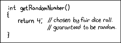
Source: XKCD #221
Key Takeaways
Key Takeaways
- Choice of probability distribution can have large impacts on uncertainty and risk estimates: try not to use distributions just because they’re convenient.
- Monte Carlo: Estimate expected values of functions using simulation.
- Monte Carlo error is on the order \(1/\sqrt{n}\), so not great if more direct approaches are available and tractable.
Upcoming Schedule
Next Classes
Friday: Simple Climate Models and Uncertainty
Next Week: Prescriptive Models and Intro to Optimization